A Problem of Fourier Analysis: Approximating Band- and Time-limited Functions | 12/18/2024
Forewarning
This problem and its proof is almost exactly from the textbook Ten Lectures on Wavelets that I read through this fall with my Directed Reading Program mentor and applied math PhD student Jack Luong. However, I am rewriting it to share here because I loved reading through its proof with Jack so much that I centered my end-of-quarter presentation on it. The balance of surprise and derivation, of application and rigor is beautiful. Because here it is cut away from a series of lectures, I warn that this proof relies on results which we must take as blackboxes. As much as I would like this problem's solution to seem like you could have derived it yourself, perhaps this is a lesson in the importance of learning the work of mathematicians before us.
A more ambitious motive is that I have changed some of the flow because I believe that I can explain it better than the renowned author of the book. You can be the judge of how well I did.
The Problem
To give context, this problem was worked on by many researchers until it was elegantly solved by H. Landau, H. Pollak, and D. Slepian in their series of papers Slepian and Pollak (1961), and Landau and Pollak in (1961, 1962).
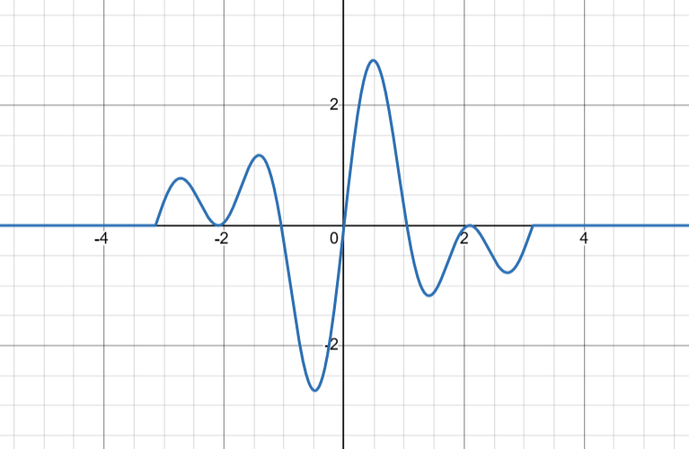
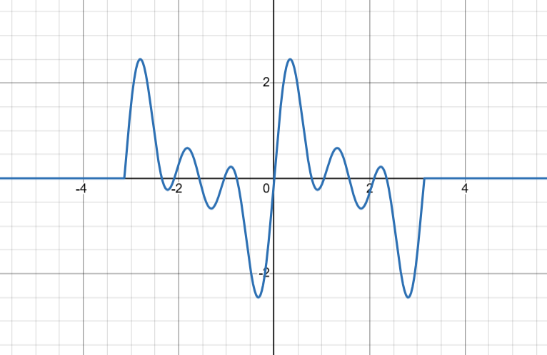
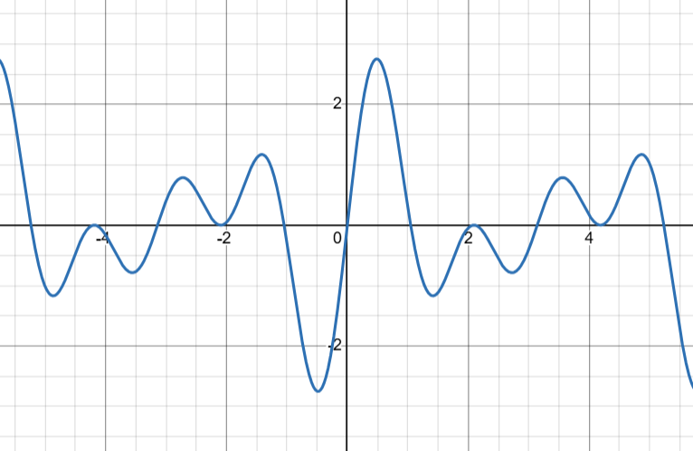
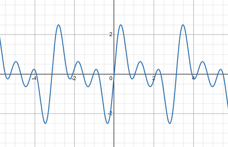
We want to model the situation in which a signal's transmission cuts off frequencies outside a certain interval and also lasts for a finite time. In all practical purposes, this is what matters; we don't really care about frequencies of signals that exceed or drop below a certain threshold, especially if it is an audio signal, and neither do we consider a signal at the beginning of the universe nor track it until the end of time. So this looks like as follows:
Signal $f$ in time domain.
Signal $\hat{f}$ in frequency domain.
For the engineers out there, the band-limiting is equivalent to passing this signal through an ideal-low pass filter. For those familiar with convolutions, mathematically this looks like multiplying a signal by the rectangular function in the frequency domain or, equivalently, convolving a sinc function with its impulse response in the time domain.
However, the catch is that no such function exists. A theorem that implies the Heisenberg uncertainty principle states that a real-valued function and its Fourier transform cannot both have compact support. Underlying this is the general Fourier analysis uncertainty principle that a narrow function has a wide Fourier transform and a wide function has a narrow Fourier transform. Hence, our quest begins to approximate this phenomenon in some way, to find which signals are most closely band- and time-limited.
The Quest
We model the time-limiting and band-limiting process by letting $Q_T, P_\Omega$ be orthogonal projection operators in $L^2(\R)$ (orthogonal meaning this preserves the inner product, and a projection characterized by $T^2 = T$) defined by
$$(Q_T f)(x) = f(x) \text{ for } |x| < T, \quad (Q_T f)(x) = 0 \text{ for } |x| > T,$$
and
$$\widehat{(P_\Omega f)} (x) = \hat{f}(\xi) \text{ for } |\xi| < \Omega, \quad \widehat{(P_\Omega f)} (x) = 0 \text{ for } |\xi| > \Omega$$
Hence, if $f$ is our signal, the function $P_\Omega Q_T f$ is the time-limiting and band-limited signal.
Then when is it true that $P_\Omega Q_T f \approx f$? How well $P_\Omega Q_T f$ actually represents the function $f$ can be measured by how close the ratio $||P_\Omega Q_T f||^2/||f||^2$ is to $1$, where this norm is the standard $L^2$-norm. Intuitively, this measures the total energy loss of time- and band-limiting the signal. After manipulations, we discover this is equal to $\left< Q_T P_\Omega Q_T f, f\right> / ||f||^2$ because
$$
\begin{align*}
|| P_\Omega Q_T f ||^2 &= \left< P_\Omega Q_T f, P_\Omega Q_T f \right>\\
&= \left< P_\Omega Q_T f, Q_T f \right>\\
&= \left< Q_T P_\Omega Q_T f, f \right>
\end{align*}
$$
where the first equality follows because both $P_\Omega$ and $Q_T$ are self-adjoint and because applying the projection operator again is itself, and the second equality follows again because $Q_T$ is self-adjoint. To calculate this inner product, we defer to the higher powers for knowledge, using the first blackbox.
Higher Power 1.
The quotient $\left< T f, f \right>/||f||^2$ is the Rayleigh quotient of a linear operator $T$ which is known how to be calculated from its eigenvalues.
In particular, if $T$ is a symmetric operator, the Rayleigh quotient is equal to the largest eigenvalue of $T$.
Since the $Q_T P_\Omega Q_T$ operator is symmetric (which follows from being real and self-adjoint, since a symmetric operator is defined as one that $\left< u, Av \right> = \left< Au, v \right> $), this quotient is equal to its largest eigenvalue.
To compute this, we write $Q_T P_\Omega Q_T f$ more explicitly. A signal $f$ after the first application of $Q_T$ looks like
$$(Q_T f)(x) =
\begin{cases}
f(x) & \text{ if } |x| < T\\
0 & \text{ if } |x| > T
\end{cases}
$$
Now to see what happens when we apply $P_\Omega$, we shall need the following important result about reconstructing functions with compactly supported Fourier transform.
Higher Power 2.
Let $B_\Omega = \{ f \in L^2(\R) : \text{support } \hat{f} \subset [-\Omega, \Omega] \}$. If $f \in B_\Omega$, then
$$f(x) = \int f(y) \displaystyle{\frac{\sin \Omega (x - y)}{\pi (x - y)} } dy$$
We can now write the operator $Q_T P_\Omega Q_T$ as
$$(Q_T P_\Omega Q_T f)(x) =
\begin{cases}
\int_{-T}^T f(y) \displaystyle{\frac{\sin \Omega (x - y)}{\pi (x - y)} } dy & \text{ if } |x| < T\\
0 & \text{ if } |x| > T
\end{cases}$$
where the last application of $Q_T$ restricts the bounds over which we integrate.
Then to find the largest eigenvalue of the operator, the last and largest highest power is bestowed upon us: we are handed another operator that commutes with ours, and we are reminded that if linear operators commute then their eigenfunctions are the same.
Higher Power 3.
The second-order differential operator commutes with $Q_T P_\Omega Q_T$, whose eigenvalues and functions are known explicitly:
$$(Af)(x) = \frac{d}{dx} (T^2 - x^2) \frac{df}{dx} - \frac{\Omega^2}{\pi^2} x^2 f(x).$$
This operator and its eigenfunctions, named the prolate spheroidal wave functions, were studied far before their connection here to band- and time-limiting was discovered. Note that because this operator is defined in terms of $T$ and $\Omega$, it is possible that they also determine its eigenfunctions. Indeed, this is true;
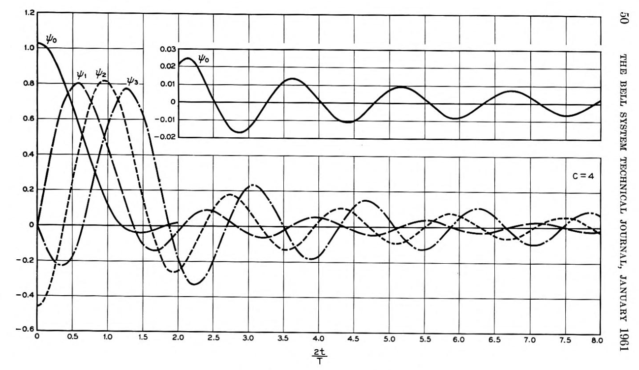
in the graph below are shown only the series of prolate spheroidal wave functions for a certain constant value of $c = 2 T \Omega$:
First four prolate spheroidal functions for $c = 2 T \Omega = 4$.
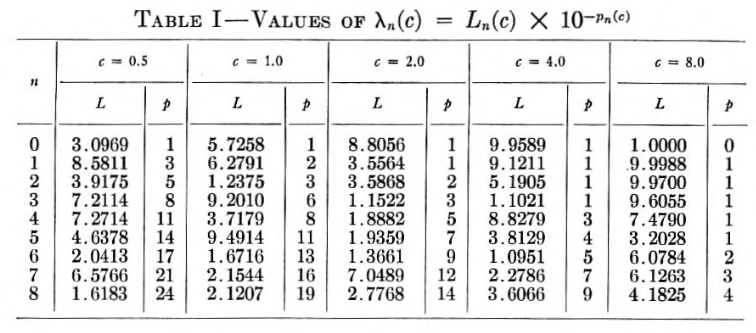
However, though the eigenfunctions between this new operator and $Q_T P_\Omega Q_T$ are the same, this says nothing about the eigenvalues. But using work that has been done before, we can index these eigenfunctions according to their eigenvalues $\lambda_n$ for $A$ in decreasing order:
Table for eigenvalues $\lambda_n$, where $c = 2 \Omega T$.
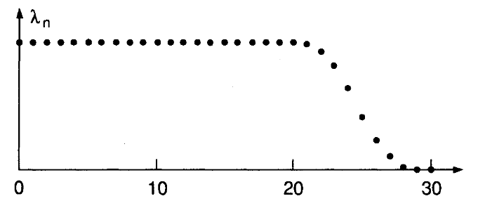
Consider the case $2 T \Omega = 8.0$. The graph of their eigenvalues is close to 1 until about $n = 3$ and rapidly drops afterwards. In a graph, we can see this in the case of $2 T \Omega / \pi = 25$:
Graph of the eigenvalues $\lambda_n$ for $Q_T P_\Omega Q_T$ for $2T\Omega/ \pi = 25$.
There are about $25$ eigenfunctions for which their corresponding eigenvalues are very close to 1. It turns out that $2 T \Omega / \pi$ is a good approximation for how many eigenfunctions can well-approximate the band- and time-limiting process. If $f = \sum_{n = 0}^{2T \Omega / \pi} c_n \psi_n$, then the band- and timelimiting process approximates the function well:
$$
\begin{align*}
Q_T P_\Omega Q_T f = (Q_T P_\Omega Q_T) \left( \sum_{n = 0}^{2T \Omega / \pi} c_n \psi_n \right) \approx 1 \cdot \left(\sum_{n = 0}^{2T \Omega / \pi} c_n \psi_n \right) = f
\end{align*}
$$
What is even more incredible is that these eigenfunctions form a complete basis in band-limited functions of $L^2(\R)$, although this fact is proved with much difficulty (Titchmarsh). So any band-limited function can be written as a linear combination of prolate spheroidal functions, and the functions that are written as linear combinations of the lower indexed PSWFs are almost exactly both band- and time-limited.
Acknowledgements
Many thanks go to Jack Luong for being my grad student mentor! His patience each week shown in dissecting proofs together, Wikipedia-ing measure theory theorems, and answering my doubts about the linear algebra theorems is something I aspire towards.
References
- Daubechies, I. (1992). Ten Lectures on Wavelets. SIAM, doi.org/10.1137/1.9781611970104.
- Dubey, Kabir. (2021). "The Fourier Uncertainty Principles." University of Chicago, math.uchicago.edu/~may/REU2021/REUPapers/Dubey.pdf.
- Georgia, The University of. "The Uncertainty Principle." University of Georgia, www.math.uga.edu/sites/default/files/uncertainty.pdf.
- Stein, E. M., & Rami Shakarchi. (2011). Fourier Analysis. Princeton University Press.
- Slepian, D., & H.O. Pollak. (1961). "Prolate Spheroidal Wave Functions, Fourier Analysis and Uncertainty - I." The Bell System Technical Journal, archive.org/details/bstj40-1-43.
- Titchmarsh, E.C. (1942). Eigenfunction Expansions Associated with Second Order Differential Equations---Part I. Oxford University Press.
Fly home, Buddy! I work alone.